Tests of a Native Windows MININEC Port

Paul McMahon VK3DIP August 2015

Back

Home

 

Back to the NEC-TIE page

As mentioned on the NEC-TIE page (link above) NEC-TIE includes a port of the MININEC code to a native windows application. This port was based on the commonly available version 3 Basic code and using the free Microsoft Visual Basic .Net development environment Visual Express 2010. Along the way I made the following changes and additions:

·        All non-integer numeric variables changed to Double Precision.

·        Constants and approximations updated to take advantage of that precision.

·        Addition of support for NEC2 style loads LD0 through LD5 (4NEC2 extensions to LD6&7 are handled as they are in 4NEC2 and converted to equivalent LD1 and LD2 respectively as a part of the NEC-TIE import process). S-Domain type loads remain.

·        Removal of support for the original MININEC .inp format, as it is superseded by the .nec format and you could only ever have one .inp file.

·        Some GUI bits to bring the data entry and editing up to modern windows norms.

 

Having done this and got it going, two questions arise ie. Does it work/give expected answers? And secondly are the changes/inclusions worth the effort?

 

The first thing to look at here, is does the change to double precision do anything for us?

 

A very useful reference to MININEC 3 is the original tech report called: “Tech Doc 938 September 1986 The new MININEC (version 3): A Mini-Numerical Electromagnetic Code”, for reference an official scan of this document is now available here:

 http://oai.dtic.mil/oai/oai?verb=getRecord&metadataPrefix=html&identifier=ADA181682

 

This document contains good discussions on the limitations to MININEC of using single precision and in particular:

 

“Numerical problems may occur in the solution when quantities become too small for the inherent accuracy of the computer.  An example is the erroneous results that can occur for very short segments. “

 

It goes on to describe a test (which it calls the Low Frequency Test) designed to identify the short segment limit. The conclusion reached from the results given in the report are:

 

“For MININEC, on a 16 bit machine in single precision, the segment length should always be greater than 10^-4 wavelengths”

 

This then is basically the origin of what has been one of the commonly quoted modelling guidelines warning against overly short segments.

 

The report also says:

 

“A change from single precision to double precision extends the validity range to even shorter segments, but significantly increases the solution time beyond acceptable run times for a 16-bit microcomputer.”

 

These days I don’t think you could get a 16 bit processor in your mobile phone if you tried, even the microcontrollers in your washing machine or car are probably better than that, let alone those in any PC or tablet. Also they are all very much faster than the ones envisioned in 1986. So I am not too worried by the acceptable run times comment. The extending of the validity down to smaller segment sizes would however be useful, particularly as having smaller segments is a well-known approach to sharp bends and other modelling problems.

 

 So I have repeated the “Low Frequency Test” using a number of available codes including the NEC-TIE port. (See Excel file download link below for details)

 

Basically the test has a one Metre long centre fed dipole in free space with ten segments and the frequency is decreased with a value of the input admittance recorded for each value. If the initial frequency was 299.79MHz then the length of the dipole in wavelengths is also one. Similarly the length of each of the ten segments is a tenth of that ie. 1/10 (or 10^-1) wave length. As the frequency is decreased this has the effect of making each segment progressively shorter in terms of a wave length.

 

The summary of these results is shown in the below graph

 

 

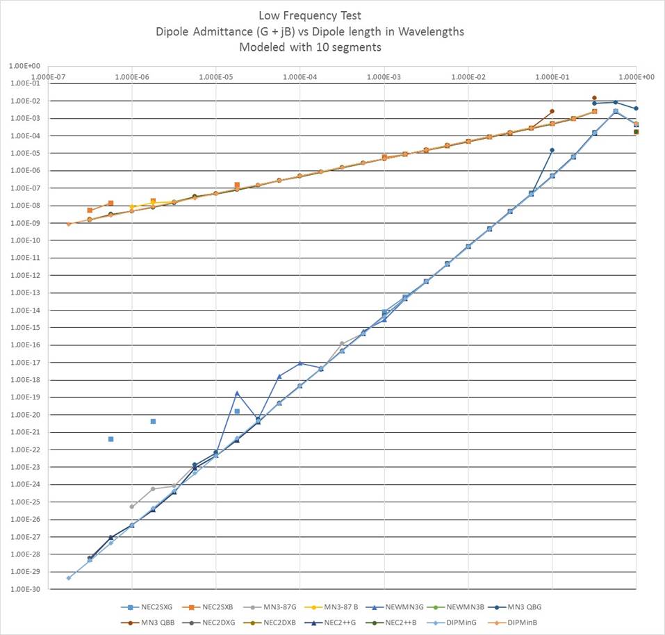
As can be seen with the dipole length below about 10^-3 (ie. segment length < 10^-4 wavelengths) I get the same strange results as quoted in the MININEC tech document for the standard single precision codes. Note even NEC2SX code has problems below this point so it does seem to be a function of precision not the code itself. Gratifyingly the double precision port of MININEC seems to deliver reasonable results well past 10^-6 (ie. with segments less than 10^-7 wavelengths long), this is as least as good as obtained with the two double precision NEC2 codes tested ie. NEC2DX and the NEC2++ ( C++ port) though to be fair to get comparable Admittance results I used 11 segments in the NEC2 cases to ensure true centre feeding, so in their cases the segment length would be dipole length divided by 11 not 10.

 

So as a result of this test I feel comfortable that the double precision is working well.

 

The second major change item is the new load types and in particular I was interested in the performance of the conductance and effective covering (ie. coated wire) loads which are not present in the original MININEC 3 code. To test this is I again took a simple model of a dipole (this time at 28.5 MHz) and progressively added the various loading effects comparing results obtained with the NEC-TIE MININEC code and NEC2DX  code (via 4NEC2) . The simplest way I found to do this was to define the antenna in 4NEC2 and then import the saved .nec file into NEC-TIE. The final (one with the lot) .nec files can be found in a link below. (both the 4nec2 file with symbols etc. and the imported NEC-TIE file with the converted loads in the one zip)

 

The summary results are shown in the below table:

 

 

 While only input impedance and efficiency are shown the patterns and gain etc. were basically identical. The agreement here is very good not only within one Ohm or so for the real component and within 2 Ohms for the imaginary, but the relative changes as each load type etc. are added are also mirrored well. The efficiency is in particularly close agreement.

 

The above is not exhaustive testing nor formal validation but is enough for me to be pretty confident using this code.

 

Files.

Excel spreadsheet of Low Frequency Test results.(Zipped)

 

.NEC files for loads test.(Zipped)

 

 

 

 

 Back

Home